Voxel-based morphometry / voxel-wise multiple regression in Python

March 02, 2021

tags:
python

I got to learn Python before using Matlab. Therefore when I needed to run my first VBM analyses, I quickly looked for a way to do this through Python scripts instead of clicking (and misclicking) hundreds of times using the graphical interface from SPM. As a summary of this past experience, here is a walkthrough to run such an analysis directly from a Python script. In particular, this recipe leverages on the nipype library. Note: it still requires Matlab and SPM but uses Python as an interface with them.

Data preparation

Let us first create the design matrix. Instead of copy-pasting it to SPM GUI, it will be just read from an Excel table.

import pandas as pd
excel_file = '/tmp/dm.xlsx'
data = pd.read_excel(excel_file, engine='openpyxl')
data.head()

id	age	sex	apoe4
/tmp/VBM/data/smwc1_10013_BBRC02_E01344.nii	59.112936	1	0
/tmp/VBM/data/smwc1_10019_BBRC_E00046.nii	63.227926	0	0
/tmp/VBM/data/smwc1_10026_BBRC02_E06149.nii	70.951403	1	1
/tmp/VBM/data/smwc1_10032_BBRC02_E07242.nii	59.750856	1	0
/tmp/VBM/data/smwc1_10034_BBRC_E02026.nii	52.443532	1	1

The first column gives a list of paths to all the NIfTI files that shall be used in the analysis.

col1 = data.columns[0]
scans = data[col1].tolist()
print('First column: %s' % col1)

First column: id

The other columns will be used as regressors.

names = list(data.columns[1:])
vectors = [data[e].tolist() for e in names]
print('Regressors in the model: %s' % str(names))

Regressors in the model: [age, sex, apoe4]

Contrasts are then defined as tuples. Each tuple follows the format: contrast name, type of statistical test, names of the columns to be used, weighting factors.

contrasts = []
cont1 = ('Effect of age (+)', 'T', ['age'], [1])
cont2 = ('Effect of age (-)', 'T', ['age'], [-1])
contrasts.append(cont1)
contrasts.append(cont2)

Now we are ready to build the analysis workflow.

Building the workflow

The workflow is composed of 3 consecutive nodes: first we design the model ("modeldesign"), then we estimate the model parameters ("estimatemodel") and finally we estimate the contrasts ("estimatecontrasts"').

The covariates need to be passed to the workflow in a certain format, which is easily achieved based on the previously prepared variables names and vectors.

covariates = []

centering = [1] * len(names)
for name, v, c in zip(names, vectors, centering):
    covariates.append(dict(name=name, centering=c, vector=v))

We may now create the nodes of the workflow. The first one (we called it "modeldesign") takes here the list of normalized scans, the covariates and some mask to restrict the area of the analysis.

import nipype.interfaces.spm as spm

explicit_mask = '/path/to/MNI_T1_brain_mask.nii'
model = spm.model.MultipleRegressionDesign(in_files=scans,
                                           user_covariates=covariates,
                                           explicit_mask_file=explicit_mask,
                                           use_implicit_threshold=True)

Then we create the two other nodes.

est = spm.EstimateModel(estimation_method={'Classical': 1})
con = spm.EstimateContrast(contrasts=contrasts,
                             group_contrast=True)

The workflow itself is defined as follows:

import nipype.pipeline.engine as pe

analysis_name = 'vbm_analysis'
w = pe.Workflow(name=analysis_name)
w.base_dir = '/path/to/destination_dir'

n1 = pe.Node(model, name='modeldesign')
n2 = pe.Node(est, name='estimatemodel')
n3 = pe.Node(con, name='estimatecontrasts')

We then need to connect the I/O across nodes, as each node may take as inputs the outputs of the previous.

w.connect([(n1, n2, [('spm_mat_file', 'spm_mat_file')]),
           (n2, n3, [('spm_mat_file', 'spm_mat_file'),
                     ('beta_images', 'beta_images'),
                     ('residual_image', 'residual_image')]), ])

We may finally configure some available options.

w.config['execution']['stop_on_first_rerun'] = True
w.config['execution']['remove_unnecessary_outputs'] = False

We now have a fully-defined workflow. It is now ready to run.

w.run()

The process should go through each node consecutively. Data from the workflow execution will be stored in the destination folder defined earlier (w.base_dir). Once completed, we may start reviewing the results.

The following function summarizes all the previously listed steps, taking a list of scans, regressors, regressor names, an explicit mask and a destination folder as inputs. Note the prior configuration of the path to Matlab and the default Matlab command to be used. The function returns a workflow that should be ready to run.

import nipype.interfaces.spm as spm
import nipype.pipeline.engine as pe
from nipype.interfaces.matlab import MatlabCommand

matlab_cmd = '/usr/local/MATLAB/R2020b/bin/matlab'
spm.SPMCommand.set_mlab_paths(matlab_cmd=matlab_cmd)
MatlabCommand.set_default_matlab_cmd('matlab -nodesktop -noplash')

def build_workflow(scans, vectors, names, contrasts, destination_folder,
                   explicit_mask, analysis_name='analysis',
                   verbose=True):
    ''' Build a Nipype pipeline for voxelwise multiple regression analysis
    on a set of scans, using an Excel sheet as design matrix (columns in
    'names') and a given explicit mask.

    The whole analysis will be performed in the directory 'destination_folder'.
    '''

    print(['Analysis name:', analysis_name])

    if verbose:
        print(['Scans (%s):' % len(scans), scans])
        print(['Vectors (%s)' % len(vectors)])
        print(['Names (%s):' % len(names), names])
        print(['Contrasts (%s):' % len(contrasts), contrasts])

    covariates = []

    centering = [1] * len(names)
    for name, v, c in zip(names, vectors, centering):
        covariates.append(dict(name=name, centering=c, vector=v))

    model = spm.model.MultipleRegressionDesign(in_files=scans,
                                               user_covariates=covariates,
                                               explicit_mask_file=explicit_mask,
                                               use_implicit_threshold=True)

    est = spm.EstimateModel(estimation_method={'Classical': 1})
    con = spm.EstimateContrast(contrasts=contrasts,
                               group_contrast=True)

    # Creating Workflow
    w = pe.Workflow(name=analysis_name)
    w.base_dir = destination_folder

    n1 = pe.Node(model, name='modeldesign')
    n2 = pe.Node(est, name='estimatemodel')
    n3 = pe.Node(con, name='estimatecontrasts')

    w.connect([(n1, n2, [('spm_mat_file', 'spm_mat_file')]),
               (n2, n3, [('spm_mat_file', 'spm_mat_file'),
                         ('beta_images', 'beta_images'),
                         ('residual_image', 'residual_image')]), ])
    w.config['execution']['stop_on_first_rerun'] = True
    w.config['execution']['remove_unnecessary_outputs'] = False
    return w

Reviewing the results

The execution data from a previous workflow can be accessed directly from the created object.

n1 = w.get_node('modeldesign')
n3 = w.get_node('estimatecontrasts')

If the workflow was executed previously, or in a separate terminal, it is still possible to retrieve this information by recreating the workflow. The process will take the information from the prior execution.

w = build_workflow(scans, vectors, names, contrasts, destination_folder,
                   explicit_mask, analysis_name, verbose=True):
n1 = w.get_node('modeldesign')
n3 = w.get_node('estimatecontrasts')
print('# of scans included in the analysis:', len(n1.inputs.in_files))

# of scans included in the analysis: 379

We may also review the estimated contrasts from node #3 ("estimatecontrasts"'):

columns = ['contrast name', 'contrast type', 'covariate names',
           'covariate weights']

df = pd.DataFrame(list(n3.inputs.contrasts),
                  columns=columns)

contrast name	contrast type	covariate names	covariate weights
Effect of age (+)	T	[age]	[1.0]
Effect of age (-)	T	[age]	[-1.0]

Statistical maps may be rendered e.g. using nilearn:

from nilearn import plotting, image
import os.path as op

for i in range(1, len(n3.inputs.contrasts) + 1):
    output_dir = op.join(destination_folder, n3._id)

    # We look for the spmT maps and keep the positive values only
    img = op.join(output_dir, 'spmT_00%02d.nii'%i)
    img = image.math_img("np.ma.masked_less(img, 0)", img=img)

    plotting.plot_stat_map(img, threshold=3.10, display_mode='z',
                           cut_coords=range(4,32,2))

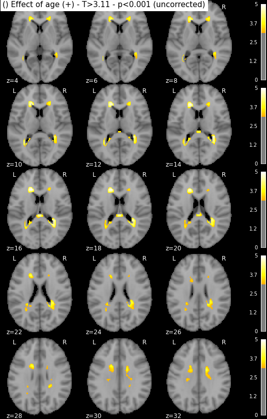
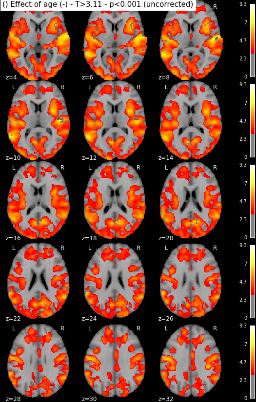
example_nilearn1 example_nilearn2

Disclaimer: in reality those snapshots were generated with another piece of code that accounts for titles and multiple lines. The interested reader might find more information here, though documentation could be much updated.

Finally, AAL users may be interested in collecting some statistics from these maps thanks to the (possibly rusty) pyAAL module. (Mode 0: Local Maxima Labeling - 1: Extended Local Maxima Labeling - 2: Cluster Labeling). Another fine Matlab-less option is atlasreader.

import pyAAL

spm_mat_file = '/tmp/dm/estimatecontrasts/SPM.mat'
out = pyAAL.pyAAL(spm_mat_file, 1, k=10, mode=2,
                  aal_nii='/path/to/ROI_MNI_V5.nii',
                  matlab_cmd='matlab')
pyAAL.to_dataframe(out)

	x,y,z	nom du label	% Cluster	Nb Vx Cluster	% Label	Nb Vx Label
0	-16 26 16	OUTSIDE	99.41	1016	0.00	0
1	-16 26 16	Caudate_L	0.59	1016	0.26	962
2	32 -42 15	OUTSIDE	99.51	1015	0.00	0
3	32 -42 15	Precuneus_R	0.49	1015	0.06	3265
4	2 -30 18	OUTSIDE	100.00	187	0.00	0
5	-32 -51 9	OUTSIDE	98.60	573	0.00	0
6	-32 -51 9	Precuneus_L	1.40	573	0.10	3528
7	20 33 -2	OUTSIDE	99.78	461	0.00	0
8	20 33 -2	Caudate_R	0.22	461	0.04	994
9	16 -2 32	OUTSIDE	100.00	235	0.00	0
10	-24 -22 32	OUTSIDE	100.00	38	0.00	0

Please let me know if you liked this post by clicking the button below.