nisnap: easy generation of snapshots from segmentation results

Processing neuroimaging data, regardless of the algorithm/software used, usually means generating more data, such as, among other possible types of outputs, numeric endpoints and, * more images *. Modern techniques now allow to use them over large collections of data, as seen with some recent large epidemiological studies and/or clinical trials. Although those image processing methods usually go through some validation process prior to publication, their performance always depends on factors that can never be fully controlled and as such, errors are still possible.

Here we are not referring to dramatic crashes, which are easy to detect (outputs would simply be missing after the pipeline's execution) and would rather be exceptional in well-designed software. A bit less rare are the errors where the pipeline reaches the end but the results would be inaccurate locally, as it might be typically the case with segmentation techniques. This might happen for various reasons eg. quality/artifacts of/in the original data, individual subject-related traits, bias compared to the original validation dataset, etc. To date there are no fail-safe or general automatic methods to detect those errors. As a consequence, visual assessment of the segmentation quality is often required, which is hard to reconcile with large sample sizes.

Still, relying on a human to do the job using any viewer ( FSLeyes, freeview, anatomist, etc) is bound to be suboptimal, for reasons due to time costs and risk of errors (operating the viewer). In that context, prerendering static summarized representations of the segmentation results can reduce this time/risk, at the price of some reduced flexibility, as compared to using any NIfTI viewer and their control parameters.

nisnap makes the generation of these summarized versions (or snapshots) easier from any Python-based context. It includes controls for:

• opacity
• layout (figure dimensions, row size)
• plane/slice selection
• color map (down to each label, described in a Json file)
• label picking
• contours/solid color rendering
• static/animated rendering (adding a fading effect between raw image and the segmentation)

Example with FreeSurfer aseg results:

This shows how to pick some selected labels out of a label volume like FreeSurfer's aseg volume. The colormap is defined in utils/colormap.json and can be adjusted as needed. The animated mode adds a fading effect between the original image and the segmentation results. The samebox option controls the zoom/bounding box around colored voxels and makes sure it is consistent across slices.

from nisnap.utils import aseg
print(aseg.basal_ganglia_labels)

[9, 10, 11, 12, 13, 17, 18, 48, 49, 50, 51, 52, 53, 54]

from nisnap import snap
snap.plot_segment('/tmp/BBRC_E00080_aparc+aseg.mgz',
                  bg='/tmp/BBRC_E00080_nu.mgz',
                  labels=aseg.basal_ganglia_labels,
                  axes='x',
                  slices=range(173,187,3),
                  contours=True,
                  samebox=True,
                  animated=True)

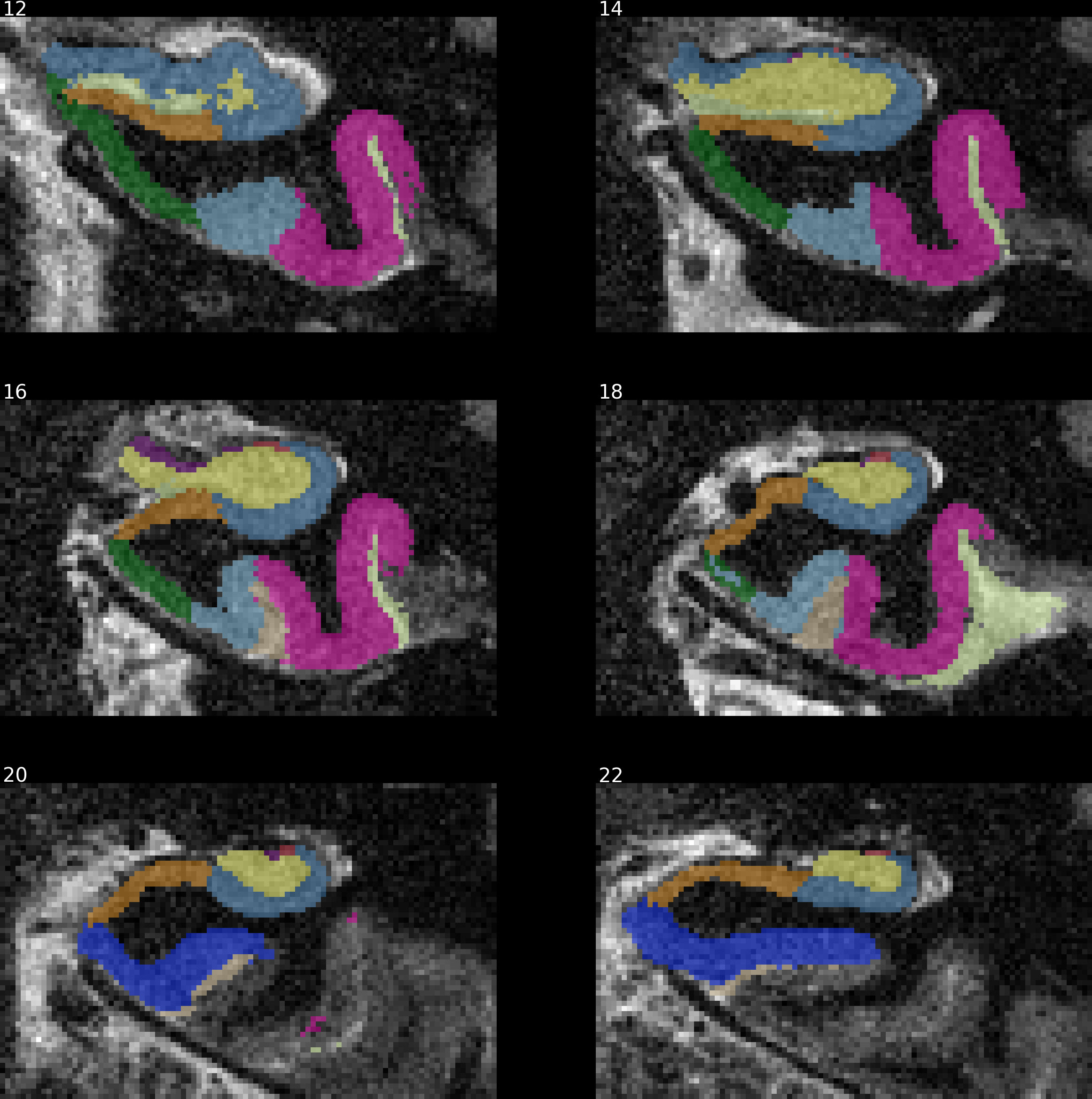
Example with ASHS (hippocampal subfield segmentation):

This example is a static one with solid colors instead of contours (using contours=False). rowsize and figsize allow to control the dimensions of the resulting figure.

from nisnap import snap
snap.plot_segment('/tmp/BBRC_E00080_ASHS_left_lfseg_corr_nogray.nii.gz',
                  bg='/tmp/BBRC_E00080_ASHS_tse.nii.gz',                  
                  axes='x',
                  contours=False,
                  samebox=True,
                  slices=range(12,24,2),
                  rowsize=2,
                  figsize=(10,10),                  
                  opacity=50)

Example with SPM:

This example combines 3 probability maps (with voxel values between 0 and 1, as produced by SPM). Layout options can be defined by axis using dictionaries.

filepaths = ['/tmp/BBRC_E00080_SPM12_SEGMENT_c1.nii.gz',
             '/tmp/BBRC_E00080_SPM12_SEGMENT_c2.nii.gz',
             '/tmp/BBRC_E00080_SPM12_SEGMENT_c3.nii.gz']

bg = '/tmp/BBRC_E00080_T1.nii.gz'
slices = {'x': list(range(130, 210, 4)),
          'y': list(range(80, 200, 6)),
          'z': list(range(50, 190, 6))}

from nisnap import snap
snap.plot_segment(filepaths,
                  bg=bg,
                  axes='xyz',
                  slices=slices,
                  samebox=True,
                  rowsize={'x': 10, 'y': 10, 'z': 8},
                  figsize={'x': (18, 4), 'y': (18, 4), 'z': (18, 5)},
                  opacity=70,                  
                  animated=True,
                  contours=False)

It also has some degree of XNAT integration, allowing to generate snapshots for a given resource on XNAT by giving its reference on the instance. Otherwise, simply passing the individual NIfTI maps, of the raw image first - if desired - then the segmentation map (or any overlay), would do the job, as shown in the previous examples.

from nisnap import xnat
xnat.plot_segment(config='/home/grg/.xnat_bsc.cfg',
                  resource_name='FREESURFER6_HIRES',
                  experiment_id='BBRC_E00080',
                  axes='x',                   
                  contours=True,
                  animated=True,
                  samebox=True,
                  slices=range(195,204,3),              
                  opacity=50)

In every case the argument savefig allows to save the result in a specific file.

nisnap may be used from Python or Jupyter Notebooks and is available as a package on PyPI (nisnap) and as a repository on GitHub.

Reference:

Operto, G., Huguet, J., nisnap v0.3.7, doi:10.5281/zenodo.4075418 (2020)